Mode Choice and Highway Assignment
Most Important Mode choice Models
-
Simple multinomial logit model
-
Incremental logit model
-
Nested logit model
-
The multinomial logit and nested logit formulations are used to estimate mode shares for most transit strategies
-
These formulations require a complete description of all modes of available or proposed highway, HOV, and transit and are extremely data-intensive.
-
The incremental logit or pivot-point formulation allows for analysis of transit improvement strategies or policies without the complete simulation of the entire transit system and its alternatives.
Mode Choice Factors
Characteristics of the trip maker
- Car availability/ownership
- Possession of a drivers license
- Household structure
- Trip chaining
- Residential density
Type of journey
- Trip purpose
- Time of day trip is taken
Characteristics of the transport facility
- Travel time: in-‐vehicle time, waiting and walking times
- Monetary cost: fares, fuel, direct costs
- Availability and cost of parking
- Comfort and convenience
- Protection and security
Key Concepts in Mode Choice
- In-Vehicle Time (IVT)
- Auto Operating Cost
- Auto Tolls
- Auto Parking Cost
- Transit Walk Time
- Transfer Time
- Number of Transfers
- Transit Fare (cents)
- Park and Ride
- Drive-Access Time
General Logit Model
$$ P_i = \frac{e^{u_i}}{\sum_{i=1}^{k}e^{u_i}} $$ $P_i$ = the probability of a traveler choosing mode i, $u_i$ = a linear function of the attributes of mode i that describe its attractiveness, also known as the utility of mode i, and
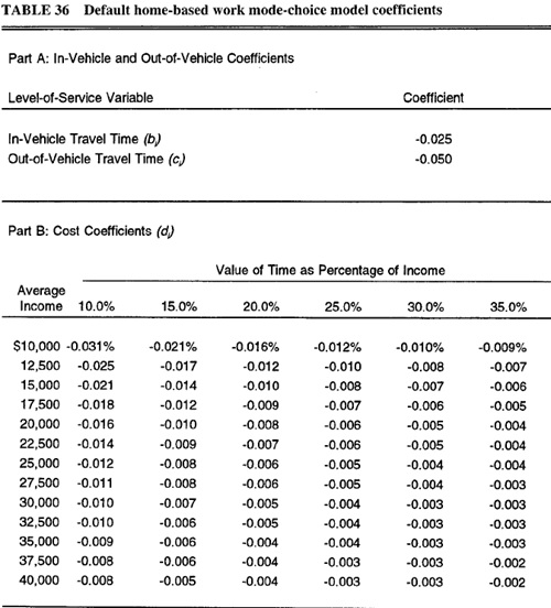
$$ u_i = a_i +b_i \times IVTT_i +c_i \times OVTT_i +d_i \times COST_i$$
Simple Multinomial Logit Model
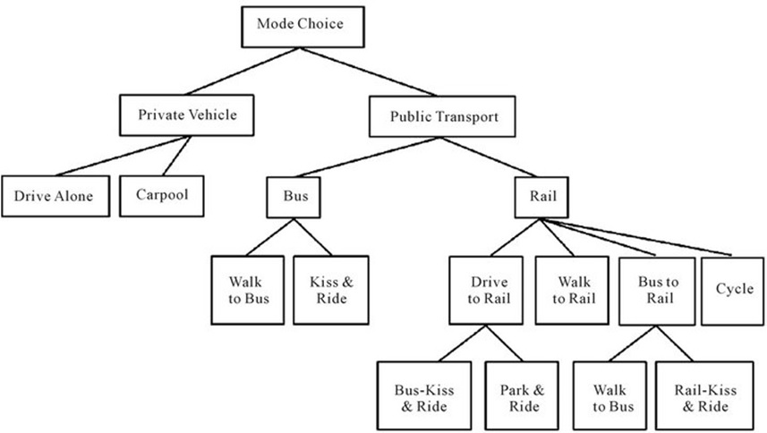
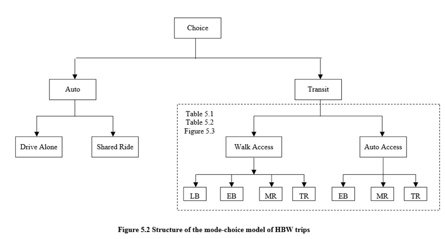
Nested Logit Model
Incremental Logit Model
Sample Mode Choice Problem
You are given the following mode choice model.
$$U_{ijm}=-1C_{ijm}+5D_T$$
where: $C_{ijm}$ = travel cost between i and j by mode m $D_T$ = dummy variable (alternative specific constant) for transit and Travel Times
Auto Travel Times
| Origin/Destination | Metropolis | New Fargo |
|---|---|---|
| Metropolis | 5 | 7 |
| New Fargo | 7 | 5 |
Transit Travel Times
| Origin/Destination | Metropolis | New Fargo |
|---|---|---|
| Metropolis | 10 | 15 |
| New Fargo | 15 | 8 |
A. Using a logit model, determine the probability of a traveler driving.
B. Using following Trip Table, how many car trips will there be?
| Origin\Destination | Metropolis | New Fargo |
|---|---|---|
| Metropolis | 9395 | 5606 |
| New Fargo | 6385 | 15665 |
Solution
A. Using a logit model, determine the probability of a traveler driving. Solution Steps
-
Compute Utility for Each Mode for Each Cell
-
Compute Exponentiated Utilities for Each Cell
-
Sum Exponentiated Utilities
-
Compute Probability for Each Mode for Each Cell
-
Multiply Probability in Each Cell by Number of Trips in Each Cell
Auto Utility: $U_{auto}$
| Origin\Destination | Metropolis | New Fargo |
|---|---|---|
| Metropolis | -5 | -7 |
| New Fargo | -7 | -5 |
Transit Utility: $U_{Trans}$
| Origin\Destination | Metropolis | New Fargo |
|---|---|---|
| Metropolis | -5 | -10 |
| New Fargo | -10 | -3 |
$e^{U_{auto}}$
| Origin\Destination | Metropolis | New Fargo |
|---|---|---|
| Metropolis | 0.0067 | 0.0009 |
| New Fargo | 0.0009 | 0.0067 |
$e^{U_{transit}}$
| Origin\Destination | Metropolis | New Fargo |
|---|---|---|
| Metropolis | 0.0067 | 0.0000454 |
| New Fargo | 0.0000454 | 0.0565 |
Sum: $e^{U_{auto}}+e^{U_{transit}}$
| Origin\Destination | Metropolis | New Fargo |
|---|---|---|
| Metropolis | 0.0134 | 0.0009454 |
| New Fargo | 0.0009454 | 0.0498 |
P(Auto) = $e^{U_{auto}}/(e^{U_{auto}}+e^{U_{transit}})$
| Origin\Destination | Metropolis | New Fargo |
|---|---|---|
| Metropolis | 0.5 | 0.953 |
| New Fargo | 0.953 | 0.12 |
P(Transit) =$e^{U_{transit}}/(e^{U_{auto}}+e^{U_{transit}})$
| Origin\Destination | Metropolis | New Fargo |
|---|---|---|
| Metropolis | 0.5 | 0.047 |
| New Fargo | 0.047 | 0.88 |
Part B
| Origin\Destination | Metropolis | New Fargo |
|---|---|---|
| Metropolis | 4697 | 5339 |
| New Fargo | 6511 | 1867 |
Highway Assignment
- Highway assignment, route choice, or traffic assignment concerns the selection of routes (alternative called paths) between origins and destinations in transportation networks.
- To determine facility needs and costs and benefits, we need to know the number of travelers on each route and link of the network (a route is simply a chain of links between an origin and destination).
- We need to undertake traffic (or trip) assignment. Suppose there is a network of highways and transit systems and a proposed addition. We first want to know the present pattern of travel times and flows and then what would happen if the addition were made.
Trip Assignment Procedure
- To estimate the volume of traffic on the links of the network and possibly the turning movements at intersections.
- To furnish estimates of travel costs between trip origins and destinations for use in trip distribution.
- To obtain aggregate network measures, e.g. total vehicular flows, total distance covered by the vehicle, total system travel time.
- To estimate zone-to-zone travel costs(times) for a given level of demand.
- To obtain reasonable link flows and to identify heavily congested links.
- To estimate the routes used between each origin to destination(O-D) pair.
Link Performance Function
The cost that a driver imposes on others is called the marginal cost. However, when making decisions, a driver only faces his own cost (the average cost) and ignores any costs imposed on others (the marginal cost).
$$ AverageCost=\dfrac{S_T}{Q}$$
$$ MarginalCost=\dfrac{\delta S_T}{\delta Q}$$
where $S_T$ is the total cost, and $Q$ is the flow.
BPR Link Performance Function
$$ T_f = T_o * (1+ \alpha *\left [ V/C \right ] ^ \beta)$$
$T_f$ = final link travel time
$T_o$ = original (free-flow) link travel time
$\alpha$ = coefficient (often set at 0.15)
V = assigned traffic volume
C = the link capacity
$\beta$ = exponent (often set 4.0)
Types of Assignment
- All-or-nothing assignment (AON),
- Incremental assignment,
- User equilibrium assignment (UE),
- Capacity restraint assignment,
- Stochastic user equilibrium assignment (SUE),
- System optimum assignment (SO), etc.
All-Or-Nothing Assignment
In this method the trips from any origin zone to any destination zone are loaded onto a single, minimum cost, path between them. This model is unrealistic as only one path between every O-D pair is utilized even if there is another path with the same or nearly same travel cost. Also, traffic on links is assigned without consideration of whether or not there is adequate capacity or heavy congestion; travel time is a fixed input and does not vary depending on the congestion on a link. However, this model may be reasonable in sparse and uncongested networks where there are few alternative routes and they have a large difference in travel cost.
- Step 1: find shortest paths between origin and destination zones
- Step 2: assign all trips to links comprising the shortest routes
This model may also be used to identify the desired path : the path which the drivers would like to travel in the absence of congestion. In fact, this model’s most important practical application is that it acts as a building block for other types of assignment techniques.It has a limitation that it ignores the fact that link travel time is a function of link volume and when there is congestion or that multiple paths are used to carry traffic.
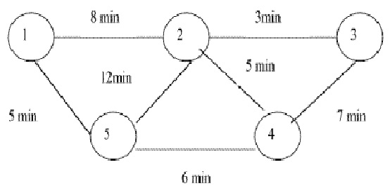
Sample Problem
*** Trips between Zones ***
| From/to | 1 | 2 | 3 | 4 | 5 |
|---|---|---|---|---|---|
| 1 | - | 100 | 100 | 200 | 150 |
| 2 | 400 | - | 200 | 100 | 500 |
| 3 | 200 | 100 | - | 100 | 150 |
| 4 | 250 | 150 | 300 | - | 400 |
| 5 | 200 | 100 | 50 | 350 | - |
Solution
| Nodes | Link | Travel | ||
|---|---|---|---|---|
| From | To | Path | Time | Volume |
| 1 | 2 | 1-2 | 8 | 100 |
| 3 | 1-2,2-3 | 11 | 100 | |
| 4 | 1-5,5-4 | 11 | 200 | |
| 5 | 1-5 | 5 | 150 | |
| 2 | 1 | 2-1 | 8 | 400 |
| 3 | 2-3 | 3 | 200 | |
| 4 | 2-4 | 5 | 100 | |
| 5 | 2-4,4-5 | 11 | 500 | |
| 3 | 1 | 3-2,2-1 | 11 | 200 |
| 2 | 3-2 | 3 | 100 | |
| 4 | 3-4 | 7 | 100 | |
| 5 | 3-4,4-5 | 13 | 150 | |
| 4 | 1 | 4-5,5-1 | 11 | 250 |
| 2 | 4-2 | 5 | 150 | |
| 3 | 4-3 | 7 | 300 | |
| 5 | 4-5 | 6 | 400 | |
| 5 | 1 | 5-1 | 5 | 200 |
| 2 | 5-4,4-2 | 11 | 100 | |
| 3 | 5-4,4-3 | 13 | 50 | |
| 4 | 5-4 | 6 | 350 | |
| Link | Volume | |||
| 1-2 | 200 | |||
| 2-1 | 600 | |||
| 1-5 | 350 | |||
| 5-1 | 450 | |||
| 2-5 | 0 | |||
| 5-2 | 0 | |||
| 2-3 | 300 | |||
| 3-2 | 300 | |||
| 2-4 | 600 | |||
| 4-2 | 250 | |||
| 3-4 | 250 | |||
| 4-3 | 350 | |||
| 4-5 | 1300 | |||
| 5-4 | 700 |
|
Incremental Assignment
Incremental assignment is a process in which fractions of traffic volumes are assigned in steps.In each step, a fixed proportion of total demand is assigned, based on all-or-nothing assignment. After each step, link travel times are recalculated based on link volumes. When there are many increments used, the flows may resemble an equilibrium assignment ; however, this method does not yield an equilibrium solution. Consequently, there will be inconsistencies between link volumes and travel times that can lead to errors in evaluation measures. Also, incremental assignment is influenced by the order in which volumes for O-D pairs are assigned, raising the possibility of additional bias in results.
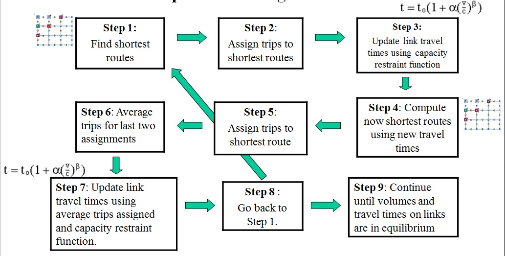
Equilbrium Assignment
To assign traffic to paths and links we have to have rules, and there are the well-known Wardrop equilibrium (1952) conditions. The essence of these is that travelers will strive to find the shortest (least resistance) path from origin to destination, and network equilibrium occurs when no traveler can decrease travel effort by shifting to a new path. These are termed user optimal conditions, for no user will gain from changing travel paths once the system is in equilibrium.
The user optimum equilibrium can be found by solving the following nonlinear programming problem $$ min \displaystyle \sum_{a} \displaystyle\int\limits_{0}^{v_a}S_a(Q_a), dx $$
subject to: $$ Q_a=\displaystyle\sum_{i}\displaystyle\sum_{j}\displaystyle\sum_{r}\alpha_{ij}^{ar}Q_{ij}^r$$ $$ sum_{r}Q_{ij}^r=Q_{ij}$$ $$ Q_a\ge 0, Q_{ij}^r\ge 0$$
where $Q_{ij}^r$ is the number of vehicles on path r from origin i to destination j. So constraint (2) says that all travel must take place: i = 1 … n; j = 1 … n $S_a(Q_a)$ is the average travel time for a vehicle on link a $\alpha_{ij}^{ar}$ = 1 if link a is on path r from i to j ; zero otherwise.
So constraint (1) sums traffic on each link. There is a constraint for each link on the network. Constraint (3) assures no negative traffic.
Transit Assignment
There are also methods that have been developed to assign passengers to transit vehicles. In an effort to increase the accuracy of transit assignment estimates, a number of assumptions are generally made. Examples of these include the following:
- All transit trips are run on a set and predefined schedule that is known or readily available to the users.
- There is a fixed capacity associated with the transit service (car/trolley/bus capacity).