Trip Generation and Trip Distribution
Fundamentals of Trip Generation
- Every trip has two ends, and we need to know where both of them are. Because land use can be divided into two broad category (residential and non-residential) we have models that are household based and non-household based.
- Trip generation is thought of as a function of the social and economic attributes of households
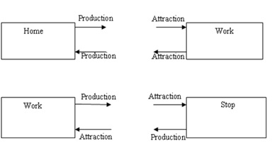
- The first part is determining how many trips originate in a zone and the second part is how many trips are destined for a zone aka “productions” and attractions Production and attractions differ from origins and destinations. Trips are produced by households even when they are returning home (that is, when the household is a destination).
Actvities for Trip Generation
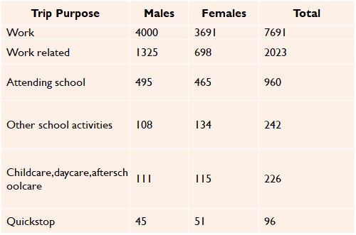
- Trips are categorized by purposes, the activity undertaken at a destination location.
- Major activities are home, work, shop, school, eating out, socializing, recreating, and serving passengers (picking up and dropping off).
- There are numerous other activities that people engage on a less than daily or even weekly basis, such as going to the doctor, banking, etc. Often less frequent categories are dropped and lumped into the catchall “Other”.
Specifying models
The number of trips originating from or destined to a purpose in a zone are described by trip rates (a cross-classification by age or demographics is often used) or equations.
Home Trips
$$T_h = f(housing \ units, household \ size, age, income, accessibility, vehicle \ ownership)$$
Work Trips
$$T_w = f(jobs(area \ of \space \ by \ type, occupancy \ rate) )$$
Shopping Trips
$$T_s = (number \ of \ retail workers, type \ of \ retail, area, location, competition)$$
Estimating Models
Home-end
-
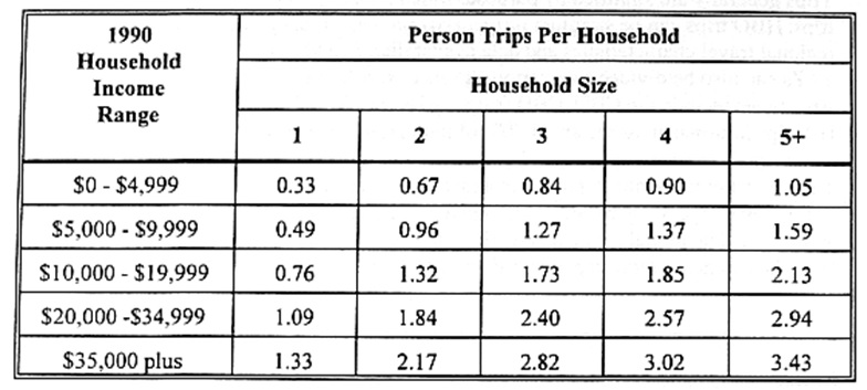
To estimate trip generation at the home end, a cross-classification model can be used. This is basically constructing a table where the rows and columns have different attributes, and each cell in the table shows a predicted number of trips, this is generally derived directly from data.
-
In the example cross-classification model: The dependent variable is trips per person. The independent variables are dwelling type (single or multiple family), household size (1, 2, 3, 4, or 5+ persons per household), and person age.
Non-home-end
- The trip generation rates for both “work” and “other” trip ends can be developed using Ordinary Least Squares (OLS) regression relating trips to employment by type and population characteristics.
- The variables used in estimating trip rates for the work-end are Employment in Offices ($E_{off}$) , Retail($E_{ret}$) , and Other($E_{oth}$)
A typical form of the equation can be expressed as:
$$T_{D,i} = a_1 E_{off,i} + a_2 E_{oth,i} + a_3 E_{ret,i}$$
$T_{D,i}$ - Person trips attracted per worker in Zone k $E_{off,i}$ - office employment in the ith zone $E_{oth,i}$ - other employment in the ith zone $E_{ret,i}$ - retail employment in the ith zone $a_1,a_2,a_3$ - model coefficients
Normalization
- For each trip purpose (e.g. home to work trips), the number of trips originating at home must equal the number of trips destined for work. Two distinct models may give two results.
- There are several techniques for dealing with this problem. One can either assume one model is correct and adjust the other, or split the difference.
- It is necessary to ensure that the total number of trip origins equals the total number of trip destinations, since each trip interchange by definition must have two trip ends.
The rates developed for the home end are assumed to be most accurate,
The basic equation for normalization:
Sample Problems
Problem 1
Planners have estimated the following models for the AM Peak Hour
$$T_{O,i}=1.5∗H_{i}$$ $$T_{D,j} =(1.5∗E_{off,j})+(1∗E_{oth,j})+(0.5∗E_{ret,j})$$ Where:
$T_{O,i}$ = Person Trips Originating in Zone i
$T_{D,j}$ = Person Trips Destined for Zone j
$H_{i}$ = Number of Households in Zone i
You are also given the following data
Data
| Variable | Metropolis | New Town |
|---|---|---|
| $H$ | 10000 | 15000 |
| $E_{off}$ | 8000 | 10000 |
| $E_{oth}$ | 3000 | 5000 |
| $E_{ret}$ | 2000 | 1500 |
A. What are the number of person trips originating in and destined for each city?
B. Normalize the number of person trips so that the number of person trip origins = the number of person trip destinations. Assume the model for person trip origins is more accurate.
Answer 1
A. What are the number of person trips originating in and destined for each city?
Solution to Trip Generation Problem Part A
| Households $H_{i}$ | Office Employees $E_{off}$ | Other Employees $E_{oth}$ | Retail Employees $E_{ret}$ | Origins $T_{O,i} = 1.5 * H_{i}$ | Destinations $T_{D,j} =(1.5∗E_{off,j})+(1∗E_{oth,j})+(0.5∗E_{ret,j})$ | |
|---|---|---|---|---|---|---|
| Metropolis | 10000 | 8000 | 3000 | 2000 | 15000 | 16000 |
| New Town | 15000 | 10000 | 5000 | 1500 | 22500 | 20750 |
| Total | 25000 | 18000 | 8000 | 3000 | 37500 | 36750 |
B. Normalize the number of person trips so that the number of person trip origins = the number of person trip destinations. Assume the model for person trip origins is more accurate.
Use:
Solution to Trip Generation Problem Part B
| Origins $T_{O,i}$ | Destinations $T_{D,j}$ | Adjustment Factor | Normalized Destinations ${T}'_{D,j}$ | Rounded | |
|---|---|---|---|---|---|
| Metropolis | 15000 | 16000 | 1.0204 | 16326.53 | 16327 |
| New Town | 22500 | 20750 | 1.0204 | 21173.74 | 21173 |
| Total | 37500 | 36750 | 1.0204 | 37500 | 37500 |
Problem 2
Modelers have estimated that the number of trips leaving Rivertown ( TO ) is a function of the number of households (H) and the number of jobs (J), and the number of trips arriving in Marcytown ( TD ) is also a function of the number of households and number of jobs.
$$T_{O}=1{H}+0.1{J};R^2=0.9$$ $$T_{D}=0.1{H}+1{J};R^2=0.5$$ Assuming all trips originate in Rivertown and are destined for Marcytown and:
Rivertown: 30000 H, 5000 J
Marcytown: 6000 H, 29000 J
Determine the number of trips originating in Rivertown and the number destined for Marcytown according to the model.
Which number of origins or destinations is more accurate? Why?
Answer 2
Determine the number of trips originating in Rivertown and the number destined for Marcytown according to the model.
$$T_{Rivertown} =T_{O} ; T_{O}= 1(30000) + 0.1(5000) = 30500 trips$$
$$T_{MarcyTown}=T_D ; T_{D}= 0.1(6000) + 1(29000) = 29600 trips$$
Which number of origins or destinations is more accurate? Why?
Origins($T_{Rivertown}$) because of the goodness of fit measure of the Statistical model ($R^2=0.9$).
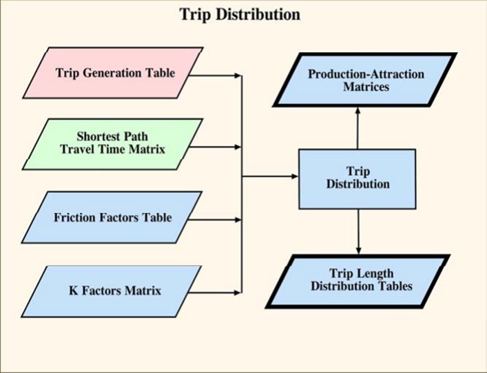
Trip Distribution
Everything is related to everything else, but near things are more related than distant things. - Waldo Tobler’s ‘First Law of Geography’
Destination Choice (or trip distribution or zonal interchange analysis), is the second component (after Trip Generation, but before Mode Choice and Route Choice) in the traditional four-step transportation forecasting model. This step matches tripmakers’ origins and destinations to develop a “trip table”, a matrix that displays the number of trips going from each origin to each destination. Historically, trip distribution has been the least developed component of the transportation planning model.
| Origin\Destination | 1 | 2 | 3 | Z |
|---|---|---|---|---|
| 1 | $T_{11}$ | $T_{12}$ | $T_{13}$ | $T_{1Z}$ |
| 2 | $T_{21}$ | |||
| Z | $T_{Z1}$ | $T_{ZZ}$ |
General Form
$$T_{ij} = T_{i} * P(T_{j})$$
Where: $T_{ij}$ = Trips from origin i to destination j.
$T_{i}$ = total trips originating at zone i
$P(T_{j})$ = probability measure that trips will be attracted to zone j
- Singly Constrained $$\sum_{i} T_{ij}= D_{i} \ or \sum_{j} T_{ij}= O_{i}$$
- Doubly Constrained $$\sum_{i} T_{ij}= D_{i} \ and \sum_{j} T_{ij}= O_{i}$$
Work trip distribution is the way that travel demand models understand how people take jobs. There are trip distribution models for other (non-work) activities, which follow the same structure.
Friction Factor Model
- Friction factors express the effect that travel that travel time has on the number of trips traveling between two zones.
Exponential
$$f(C_{ij}) = e ^ {-c(c_{ij})} \ c >0$$
Inverse Power
$$f(C_{ij}) = c_{ij} ^ {-b} \ b >0$$
Gamma
$$f(C_{ij}) = a \ X \ c_{ij} ^ {-b} \ X\ e ^ {-c(c_{ij})} \ a >0, \ b >0, \ c >0$$
Friction factors were developed using a gamma function to estimate the friction factors and application of the trip distribution model to identify the best-fit for the average trip length and trip length frequency distributions.
Fratar Model
The simplest trip distribution models (Fratar or Growth models) simply extrapolate a base year trip table to the future based on growth,
$$T_{ij,y+1} = g * T_{ij,y}$$
where:
- $T_{ij,y}$ - Trips from i to j in year y
- g - growth factor
Fratar Model takes no account of changing spatial accessibility due to increased supply or changes in travel patterns and congestion.
Gravity Model
The Gravity Model assumes that the number of trips between two zones is
- directly proportional to the trips produced and attracted to both zones, and
- inversely proportional to the travel time between the zones. The distance decay factor of ${ distance^{-1}}$ has been updated to a more comprehensive function of generalized cost, which is not necessarily linear - a negative exponential tends to be the preferred form.
- The gravity model is much like Newton’s theory of gravity. The gravity model assumes that the trips produced at an origin and attracted to a destination are directly proportional to the total trip productions at the origin and the total attractions at the destination.
While the gravity model is very successful in explaining the choice of a large number of individuals, the choice of any given individual varies greatly from the predicted value. As applied in an urban travel demand context, the disutilities are primarily time, distance, and cost, although discrete choice models with the application of more expansive utility expressions are sometimes used, as is stratification by income or auto ownership.
Mathematically, the gravity model often takes the form:
$$T_{ij}=r_is_jT_{O,i}T_{D,j}F(C_{ij})$$
$$\displaystyle \sum{j}T_{ij}=T_{O,i}, \displaystyle \sum{i} T_{ij} = T_{D,j}$$
$$r_i = (\displaystyle \sum{j} s_jT_{D,j}f(C_{ij}))^{-1}$$
$$s_j=(\displaystyle \sum{i} r_iT_{O,i}f(C_{ij}))^{-1}$$
where
$T_{ij}$ = Trips between origin i and destination j
$T_{O,i}$ = Trips originating at i
$T_{D,j}$ = Trips destined for j
$C_{ij}$ = travel cost between i and j
$r_i,s_j$ = balancing factors solved iteratively.
$f$ = impedance or distance decay factor
It is doubly constrained so that Trips from i to j equal number of origins and destinations.
Balancing Matrix
Balancing a matrix can be done using what is called the Furness Method, summarized and generalized below.
- Assess Data, you have $T_{O,i} , T_{D,j} , C_{ij}$
- Compute f(Cij) , e.g.
$$f(C_{ij})=C_{ij}^{-2}$$
$$f(C_{ij})=e^{\beta C_{ij}}$$
- Iterate to Balance Matrix
(a) Multiply Trips from Zone i ($T_i$) by Trips to Zone j($T_j$) by Impedance in Cell ij($f(Cij)$ for all ij
(b) Sum Row Totals $T′{O,i}$ , Sum Column Totals $T′{D,j}$
(c) Multiply Rows by $N_{O,i} =T_{O,i}/T′_{O,i}$
(d) Sum Row Totals $T′{O,i}$ , Sum Column Totals $T′{D,j}$
(e) Compare $T_{O,i}$ and $T′{O,i}$ , $T{D,j}$, $T′_{D,j}$ if within tolerance stop, Otherwise go to (f)
(f) Multiply Columns by $N_{D,j}=T_{D,j}/T′_{D,j}$
(g) Sum Row Totals $T′{O,i}$ , Sum Column Totals $T′{D,j}$
(h) Compare $T_{O,i}$ and $T′{O,i}$ , $T{D,j}$ and $T′_{D,j}$ if within tolerance stop, Otherwise go to (b)
Examples
Example 1
You are given the travel times between zones, compute the impedance matrix $f(C_{ij})$ , assuming $f(C_{ij})=C_{ij}^{-2}$
| Origin Zone | Destination Zone 1 | Destination Zone 2 |
|---|---|---|
| 1 | 2 | 5 |
| 2 | 5 | 2 |
Compute impedances ( $f(C_{ij})$ )
Solution
| Origin Zone | Destination Zone 1 | Destination Zone 2 |
|---|---|---|
| 1 | $1 \div {2^2}=0.25$ | $1 \div {5^2}=0.04$ |
| 2 | $1 \div {5^2}=0.04$ | $1 \div {2^2}=0.25$ |
Example 2
You are given the travel times between zones, trips originating at each zone (zone1 =15, zone 2=15) trips destined for each zone (zone 1=10, zone 2 = 20) and asked to use the classic gravity model $f(C_{ij})=C_{ij}^{-2}$
Travel Time OD Matrix
| Origin Zone | Destination Zone 1 | Destination Zone 2 |
|---|---|---|
| 1 | 2 | 5 |
| 2 | 5 | 2 |
Solution
(a) Compute impedances ( $f(C_{ij})$ )
Impedance Matrix
| Origin Zone | Destination Zone 1 | Destination Zone 2 |
|---|---|---|
| 1 | $1 \div {2^2}=0.25$ | $1 \div {5^2}=0.04$ |
| 2 | $1 \div {5^2}=0.04$ | $1 \div {2^2}=0.25$ |
(b) Find the trip table
Balancing Iteration 0
| Origin Zone | Trips Originating | Destination Zone 1 | Destination Zone 2 |
|---|---|---|---|
| Trips Destined | 10 | 20 | |
| 1 | 15 | 0.25 | 0.04 |
| 2 | 15 | 0.04 | 0.25 |
Balancing Iteration 1
| Origin Zone | Trips Originating | Destination Zone 1 | Destination Zone 2 | Row Total | Normalizing factor $N_{O,i} =T_{O,i}/T′_{O,i}$ |
|---|---|---|---|---|---|
| Trips Destined | 10 | 20 | |||
| 1 | 15 | 37.5 | 12 | 49.5 | 0.303 |
| 2 | 15 | 6 | 75 | 81 | 0.185 |
| Column Total | 43.5 | 87 |
Balancing Iteration 2
| Origin Zone | Trips Originating | Destination Zone 1 | Destination Zone 2 | Row Total | Normalizing factor $N_{O,i} =T_{O,i}/T′_{O,i}$ |
|---|---|---|---|---|---|
| Trips Destined | 10 | 20 | |||
| 1 | 15 | 11.36 | 3.64 | 15.0 | 1.0 |
| 2 | 15 | 1.11 | 13.89 | 15.0 | 1.0 |
| Column Total | 12.47 | 17.53 | |||
| Normalizing Factor | 0.802 | 1.141 |
Balancing Iteration 3
| Origin Zone | Trips Originating | Destination Zone 1 | Destination Zone 2 | Row Total | Normalizing factor $N_{O,i} = T_{O,i}/T^'_{O,i}$ |
|---|---|---|---|---|---|
| Trips Destined | 10 | 20 | |||
| 1 | 15 | 9.11 | 4.15 | 13.26 | 1.13 |
| 2 | 15 | 0.89 | 15.85 | 16.74 | 0.9 |
| Column Total | 10.0 | 20.0 | |||
| Normalizing Factor | 1.0 | 1.0 |
Balancing Iteration 4
| Origin Zone | Trips Originating | Destination Zone 1 | Destination Zone 2 | Row Total | Normalizing factor $N_{O,i} =T_{O,i}/T′_{O,i}$ |
|---|---|---|---|---|---|
| Trips Destined | 10 | 20 | |||
| 1 | 15 | 10.31 | 4.69 | 15.00 | 1.00 |
| 2 | 15 | 0.8 | 14.20 | 15.00 | 1.00 |
| Column Total | 11.1 | 18.9 | |||
| Normalizing Factor | 0.9 | 1.06 |
Balancing Iteration 16
| Origin Zone | Trips Originating | Destination Zone 1 | Destination Zone 2 | Row Total | Normalizing factor $N_{O,i} =T_{O,i}/T′_{O,i}$ |
|---|---|---|---|---|---|
| Trips Destined | 10 | 20 | |||
| 1 | 15 | 9.39 | 5.61 | 15.00 | 1.00 |
| 2 | 15 | 9.39 | 5.61 | 15.00 | 1.00 |
| Column Total | 10.1 | 19.99 | |||
| Normalizing Factor | 1.0 | 1.0 |
So while the matrix is not strictly balanced, it is very close, well within a 1% threshold, after 16 iterations. The threshold refers to the proximity of the normalizing factor to 1.0.
Comparison of Trip Distribution Models
| Model | Advantages | Disadvantages |
|---|---|---|
| Growth Factor | Simple, Easy to balance origin and destination trips at any zone | 1.Does not reflect changes in the frictions between zones 2. Does not reflect changes in the network |
| Gravity | Specific account of friction and interaction between zones | Requires extensive calibration, Long iterative process |